44 excel chart only show certain data labels
How to Use Cell Values for Excel Chart Labels Select the chart, choose the "Chart Elements" option, click the "Data Labels" arrow, and then "More Options." Uncheck the "Value" box and check the "Value From Cells" box. Select cells C2:C6 to use for the data label range and then click the "OK" button. The values from these cells are now used for the chart data labels. Hiding data labels for some, not all values in a series Here's a good challenge for you. I can't figure it out, and I believe it's a limitation of Excel. I have a bar graph with several data series. I know how to show the data labels for every data point in a given series. But I'm looking to show the data label for only some data points in a given series -- i.e. non-zero valued data points.
Display every "n" th data label in graphs - Microsoft Community you can use a free tool created by Rob Bovey, called the XY Chart Labeler. With this tool you can assign a range of cells to be the labels for chart series, instead of the Excel defaults. Using a formula, you can have a text show up in every nth cell and then use that range with the XY Chart Labeler to display as the series label.
Excel chart only show certain data labels
Excel chart not showing all data selected - Microsoft Community Double-click any of the dates along the x-axis, or the x-axis itself. In the Format Axis taskpane, look at the Minimum and Maximum. If you see Reset next to the box, click it to make the bound automatic (it should read Auto after that) --- Kind regards, HansV Report abuse 82 people found this reply helpful · Dynamically Label Excel Chart Series Lines - My Online Training Hub Step 1: Duplicate the Series. The first trick here is that we have 2 series for each region; one for the line and one for the label, as you can see in the table below: Select columns B:J and insert a line chart (do not include column A). To modify the axis so the Year and Month labels are nested; right-click the chart > Select Data > Edit the ... Find, label and highlight a certain data point in Excel ... - Ablebits Select the Data Labels box and choose where to position the label. By default, Excel shows one numeric value for the label, y value in our case. To display both x and y values, right-click the label, click Format Data Labels…, select the X Value and Y value boxes, and set the Separator of your choosing: Label the data point by name
Excel chart only show certain data labels. Add data labels to chart but only for most recent and oldest value For a new thread (1st post), scroll to Manage Attachments, otherwise scroll down to GO ADVANCED, click, and then scroll down to MANAGE ATTACHMENTS and click again. Now follow the instructions at the top of that screen. New Notice for experts and gurus: Data Labels - I Only Want One - Google Groups Use ribbon Chart Tools > Layout > Labels > Data Labels > More Data Label Options. You can now apply specific label type to selected point only. Another way would be to add a dummy series that only... Excel tutorial: Dynamic min and max data labels To make the formula easy to read and enter, I'll name the sales numbers "amounts". The formula I need is: =IF (C5=MAX (amounts), C5,"") When I copy this formula down the column, only the maximum value is returned. And back in the chart, we now have a data label that shows maximum value. Now I need to extend the formula to handle the minimum value. Only Label Specific Dates in Excel Chart Axis - YouTube Date axes can get cluttered when your data spans a large date range. Use this easy technique to only label specific dates.Download the Excel file here: https...
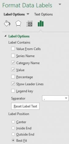
Solved: Show data label only to one line - Power BI This is a bit of a hack but you can make a copy of the graph so you have two identical graphs (make sure both the x and y axis are fixed to the same min/max). On one graph remove all of the lines you don't want to display the data and turn data labels on for this graph. On the second graph remove all of the lines you do want with data. How to Change Excel Chart Data Labels to Custom Values? First add data labels to the chart (Layout Ribbon > Data Labels) Define the new data label values in a bunch of cells, like this: Now, click on any data label. This will select "all" data labels. Now click once again. At this point excel will select only one data label. Go to Formula bar, press = and point to the cell where the data label ... Add data labels and callouts to charts in Excel 365 - EasyTweaks.com The steps that I will share in this guide apply to Excel 2021 / 2019 / 2016. Step #1: After generating the chart in Excel, right-click anywhere within the chart and select Add labels . Note that you can also select the very handy option of Adding data Callouts. Change the format of data labels in a chart To get there, after adding your data labels, select the data label to format, and then click Chart Elements > Data Labels > More Options. To go to the appropriate area, click one of the four icons ( Fill & Line, Effects, Size & Properties ( Layout & Properties in Outlook or Word), or Label Options) shown here.
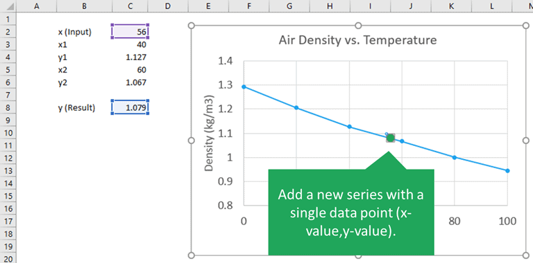
How to Only Show Selected Data Points in an Excel Chart Download Free Sample Dashboard Files here: on how to show or hide specific data points i... Creating a chart with dynamic labels - Microsoft Excel 2016 1. Right-click on the chart and in the popup menu, select Add Data Labels and again Add Data Labels : 2. Do one of the following: For all labels: on the Format Data Labels pane, in the Label Options, in the Label Contains group, check Value From Cells and then choose cells: For the specific label: double-click on the label value, in the popup ... charts - Excel, giving data labels to only the top/bottom X% values ... 1) Create a data set next to your original series column with only the values you want labels for (again, this can be formula driven to only select the top / bottom n values). See column D below. 2) Add this data series to the chart and show the data labels. 3) Set the line color to No Line, so that it does not appear! 4) Volia! See Below! Share Label Specific Excel Chart Axis Dates - My Online Training Hub Steps to Label Specific Excel Chart Axis Dates. The trick here is to use labels for the horizontal date axis. We want these labels to sit below the zero position in the chart and we do this by adding a series to the chart with a value of zero for each date, as you can see below: Note: if your chart has negative values then set the 'Date Label ...
Excel Chapter 2 – Business Computers 365
Is there a way to show only specific values in x-axis of an excel chart ... 1 Answer. 1) Use a line chart, which treats the horizontal axis as categories (rather than quantities). 2) Use an XY/Scatter plot, with the default horizontal axis "turned off" and replaced with a "helper" series with vertical values of 0 and horizontal values as desired in your dataset (this is my preferred method).

How to Change Excel Chart Data Labels to Custom Values?
Excel VBA chart, show data label on last point only Try this. First it applies datalabels to ALL points, and then removes them from each point except the last one. I use the Points.Count - 1 that way the For/Next loop stops before the last point.. Sub Data_Labels() ' Data_Labels Macro Dim ws As Worksheet Dim cht as Chart Dim srs as Series Dim pt as Point Dim p as Integer Set ws = ActiveSheet Set cht = ws.ChartObjects("Menck Chart") Set srs ...
:max_bytes(150000):strip_icc()/FormattabinExcel-a653a60322174f2e8ba05398723aee3e.jpg)
Understanding Excel Chart Data Series, Data Points, and Data Labels
How to add data labels from different column in an Excel chart? Click any data label to select all data labels, and then click the specified data label to select it only in the chart. 3. Go to the formula bar, type =, select the corresponding cell in the different column, and press the Enter key. See screenshot: 4. Repeat the above 2 - 3 steps to add data labels from the different column for other data points.
34 How To Label Specific Points In Excel - Labels For You
Only chart certain values - Excel Help Forum Re: Only chart certain values Have the data you are pulling from be the result of formulas such as =IF (xyz=0,NA (),xyz) This means that in place of 0 you will have N/A and that will not be plotted on the chart (Unless it is one specific type which will still show it - Can't remember which).

Microsoft Tips with Temo!: How to Add Data Labels to an Excel 2010 Chart
Excel tutorial: How to use data labels Generally, the easiest way to show data labels to use the chart elements menu. When you check the box, you'll see data labels appear in the chart. If you have more than one data series, you can select a series first, then turn on data labels for that series only. You can even select a single bar, and show just one data label.
Excel Bar Charts - Clustered, Stacked - Template - Automate Excel
How to create Custom Data Labels in Excel Charts - Efficiency 365 Add default data labels. Click on each unwanted label (using slow double click) and delete it. Select each item where you want the custom label one at a time. Press F2 to move focus to the Formula editing box. Type the equal to sign. Now click on the cell which contains the appropriate label. Press ENTER.

Subtotals: Pivot Table/Chart | Formulas | Jan's Working with Numbers
Highlight a Specific Data Label in an Excel Chart - Peltier Tech * right click on the series, choose Change Series Chart Type from the pop up menu, and select the desired chart type. Add data labels to each line chart* (left), then format them as desired (right). * right click on the series, choose Add Data Labels from the pop up menu. Finally format the two line chart series so they use no line and no marker.
How to Create a Pivot Table in Excel - HowtoExcel.net
Add a DATA LABEL to ONE POINT on a chart in Excel Steps shown in the video above: Click on the chart line to add the data point to. All the data points will be highlighted. Click again on the single point that you want to add a data label to. Right-click and select ' Add data label ' This is the key step! Right-click again on the data point itself (not the label) and select ' Format data label '.
Fixing Your Excel Chart When the Multi-Level Category Label Option is Missing. - Excel Dashboard ...
Add or remove data labels in a chart - support.microsoft.com Click the data series or chart. To label one data point, after clicking the series, click that data point. In the upper right corner, next to the chart, click Add Chart Element > Data Labels. To change the location, click the arrow, and choose an option. If you want to show your data label inside a text bubble shape, click Data Callout.

How to hide zero data labels in chart in Excel? - ExtendOffice Sometimes, you may add data labels in chart for making the data value more clearly and directly in Excel. But in some cases, there are zero data labels in the chart, and you may want to hide these zero data labels. Here I will tell you a quick way to hide the zero data labels in Excel at once. Hide zero data labels in chart

Chart-me XLS 2.1
Find, label and highlight a certain data point in Excel ... - Ablebits Select the Data Labels box and choose where to position the label. By default, Excel shows one numeric value for the label, y value in our case. To display both x and y values, right-click the label, click Format Data Labels…, select the X Value and Y value boxes, and set the Separator of your choosing: Label the data point by name

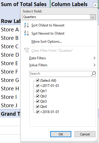
How to Add Filter to Pivot Table: 7 Steps (with Pictures)
Dynamically Label Excel Chart Series Lines - My Online Training Hub Step 1: Duplicate the Series. The first trick here is that we have 2 series for each region; one for the line and one for the label, as you can see in the table below: Select columns B:J and insert a line chart (do not include column A). To modify the axis so the Year and Month labels are nested; right-click the chart > Select Data > Edit the ...

30 How To Add Label To Excel Chart - Labels Database 2020
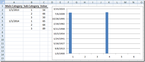
Excel chart not showing all data selected - Microsoft Community Double-click any of the dates along the x-axis, or the x-axis itself. In the Format Axis taskpane, look at the Minimum and Maximum. If you see Reset next to the box, click it to make the bound automatic (it should read Auto after that) --- Kind regards, HansV Report abuse 82 people found this reply helpful ·


How-to Use Data Labels from a Range in an Excel Chart - Excel Dashboard Templates

Show Trend Arrows in Excel Chart Data Labels

How to Make Charts and Graphs in Excel | Smartsheet
Post a Comment for "44 excel chart only show certain data labels"