42 pivot table concatenate row labels

multiple fields as row labels on the same level in pivot table Excel ... multiple fields as row labels on the same level in pivot table Excel 2016. I am using Excel 2016. I have data that lists product models along with relevant data and also production volumes by month. Part of the relevant data are about 5 common part columns with the part # that applies to each model under the appropriate column. Grouping labels and concatenating their text values (like a pivot table) Select your table; Under the POWER QUERY tab (or DATA in 2016), select "From Table" Click on the "Product" column; under the Transform tab, select "Group By" On the View tab, make sure "Formula Bar" is checked; Change the formula . FROM: = Table.Group(#"Changed Type", {"Product"}, {{"Count", each Table.RowCount(_), type number}}) TO:

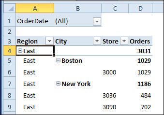
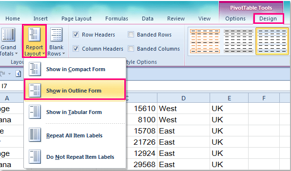
How to make row labels on same line in pivot table? Click any cell in your pivot table, and the PivotTable Tools tab will be displayed. 2. Under the PivotTable Tools tab, click Design > Report Layout > Show in Tabular Form, see screenshot: 3. And now, the row labels in the pivot table have been placed side by side at once, see screenshot:

Pivot table concatenate row labels

How to Customize Your Excel Pivot Chart Data Labels - dummies The Data Labels command on the Design tab's Add Chart Element menu in Excel allows you to label data markers with values from your pivot table. When you click the command button, Excel displays a menu with commands corresponding to locations for the data labels: None, Center, Left, Right, Above, and Below. None signifies that no data labels ... Pivot table row labels side by side - Excel Tutorials Now, let's create a pivot table ( Insert >> Tables >> Pivot Table) and check all the values in Pivot Table Fields. Fields should look like this. Right-click inside a pivot table and choose PivotTable Options…. Check data as shown on the image below. The table is going to change. The pivot table is almost ready. Spreadsheets: Problems with Pivot Table Labels - CFO To return to a normal layout of the pivot table, follow these steps: 1. Select any cell inside the pivot table. The PivotTable Tools tabs appear in the Ribbon. 2. Go to Design tab of the ribbon. 3. From the Design tab, open the Report Layout dropdown. 4.

Pivot table concatenate row labels. How to rename group or row labels in Excel PivotTable? 1. Click at the PivotTable, then click Analyze tab and go to the Active Field textbox. 2. Now in the Active Field textbox, the active field name is displayed, you can change it in the textbox. You can change other Row Labels name by clicking the relative fields in the PivotTable, then rename it in the Active Field textbox. How to add column labels in pivot table [SOLVED] Steps:-. Click any date in the Column Lables. Click Pivot table options tab on the Ribbon. In the Options Table, Click Group Field option. Click Months then click Ok. Thats it. check the attached file:-. Attached Files. PIVOT.xlsx‎ (30.3 KB, 6 views) Download. Duplicate Items Appear in Pivot Table - Excel Pivot Tables In Row 2 of the new column, enter the formula =TRIM(C2). Copy the formula down to the last row of data in the source table. If the source data is stored in an Excel Table, the formula should copy down automatically. Refresh the pivot table ; Remove the City field from the pivot table, and add the CityName field to replace it. _____ Automatic Row And Column Pivot Table Labels - How To Excel At Excel Select the data set you want to use for your table The first thing to do is put your cursor somewhere in your data list Select the Insert Tab Hit Pivot Table icon Next select Pivot Table option Select a table or range option Select to put your Table on a New Worksheet or on the current one, for this tutorial select the first option Click Ok

Pivottable Concatenate Different Row Labels Pivottable Concatenate Different Row Labels - 15 images - how to sort pivot table row labels column field labels, igoogledrive google spreadsheet sum of cells on different, how to repeat row labels for group in pivot table, strength and conditioning in swimming bb strength and, merge - Excel Pivot Table - Combine rows - Stack Overflow 1 Follow the steps - 1. Right click on any one of the dates in column 1 (dates & time). 2. Select "Group..." in the dropdown. 3. In the pop-up select "By" >>> "Days" 4. Select the "Number of days" range, in your case it would be 1. 5. Click OK. Hopefully you'll get your desired result. Share answered Sep 21, 2018 at 11:02 Nikzad Shahmardani 11 3 How to consolidate text with Pivot Table in Excel Right-click on the table name in the PivotTable Fields pane and click Add Measure. Give the measure a name and enter the formula based on your data. Then, click OK to add the measure. Once the measure is ready, move the category field ( Name) into Rows and new measure ( Abilities in our sample) into Values. The pivot table will show the results. πανεπιστημιο πατρων - Nemertes από Ε Γκίζα · 2007 — Οιπίνακες διάστασης(Dimension Tables) περιέχουν τα δεδομένα κάθε ... περιστροφή(pivot): αναπροσανατολισμόςτηςπολυδιάστατηςπροβολής ... label i και.286 σελίδες

Combining row labels in pivot table : excel - Reddit As an example if the row labels are salesman and some of the cells from the raw table have James Bond and others have bond, or JB. Each of these iteration gets its own row in the pivot table. So my question is there a way to combine these rows manually. I'm hiding averages in the pivot table so I can't simply add then all. Thanks :) Pivot Table combine rows - MrExcel Message Board The row labels of my pivot table consist of two fields in the data table: Employee ID and Employee Name. I want these to show up in one pivot table row rather than stacked: I know I could create a formula that combines the ID and Name, and then use that formula as the row label in the pivot table. Pivot table row labels in separate columns • AuditExcel.co.za Our preference is rather that the pivot tables are shown in tabular form (all columns separated and next to each other). You can do this by changing the report format. So when you click in the Pivot Table and click on the DESIGN tab one of the options is the Report Layout. Click on this and change it to Tabular form. Group or ungroup data in a PivotTable - support.microsoft.com With time grouping, relationships across time-related fields are automatically detected and grouped together when you add rows of time fields to your PivotTables. Once grouped together, you can drag the group to your Pivot Table and start your analysis.

30 Pivot Table Blank Row Label - Labels Database 2020

Pivot Table - Combine Row Labels : excel - reddit If you select In Progess, Not Attempted, and #N/A rows, the right click and hit "Group/Ungroup", you should be able to group them into an "Incomplete" Group. 2 level 2 valsimots Op · 2y Oh no way! That easy! I've been on this for hours! Thank you so very much!!! Solution Verified 2 Continue this thread More posts from the excel community 157

Importing a Hierarchy Tree Structure | Monarch Tracking

Ανάπτυξη Widgets για την Πλατφόρμα Εξόρυξης Δεδομένων ... Data Table. Paint Data. Data Info. Data Sampler. Select. Columns. Select Rows. Pivot Table. Rank. Correlations. Merge Data. Concatenate. Select by Data.113 σελίδες

Repeat Pivot Table Labels in Excel 2010 – Excel Pivot Tables

Group data in an Excel Pivot Table - Ablebits To group the data by date, right click on a date in a column or row of your PivotTable and choose Group. You can group by Seconds, Minutes, Hours, Days, Months, Quarters or Years and set the starting and ending times. For groupings like Year and Month the interval is set to 1, but for Days you can set your own interval so you can group at an ...

How to repeat row labels for group in pivot table?

Combining two+ Columns to form one Row label column in Pivot Table Select a cell in your pivot table. Press Alt, then D, then P (i.e. in succession; not all at the same time), to call up the Pivot Table Wizard. Click "" button twice. In the "Range:" box, enter the (1st)Part#-Jan range, then click "Add" button.

Repeat Pivot Table row labels • AuditExcel.co.za Pivot Tables Course

VBA code to select specific part of pivot table data That might work by copying firs the headers and then the data values after that. The code for the Row header selection is the following: ActiveSheet.PivotTables("PivotTable1").RowRange.Select. Hope this helps, Daniel van den Berg | Washington, USA | "Anticipate the difficult by managing the easy".

How to Sort Pivot Table Row Labels, Column Field Labels and Data Values with Excel VBA Macro ...

Combining two date fields into one PivotTable Row Label Hi, You will have to first rearrange your source data into a 3 column using Power Query a.k.a. Get & Transform in Excel 2016. Once done, you can easily create your desired Pivot Table. To rearrange the dataset, use the "Unpivot other columns" feature of Power Query. Here's a screenshot. Regards, Ashish Mathur. .

Pivot Table Row Labels In the Same Line - Beat Excel!

Group Pivot Table Items in Excel (In Easy Steps) - Excel Easy 1. In the pivot table, select Apple and Banana. 2. Right click and click on Group. 3. In the pivot table, select Beans, Broccoli, Carrots, Mango and Orange. 4. Right click and click on Group. Note: to change the name of a group (Group1 or Group2), select the name, and edit the name in the formula bar.

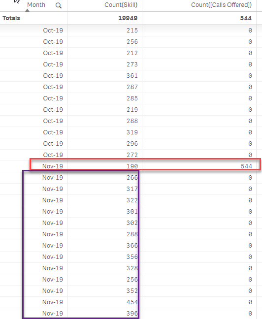
How to sum up the count measure by month and year ... - Qlik Community - 1661550

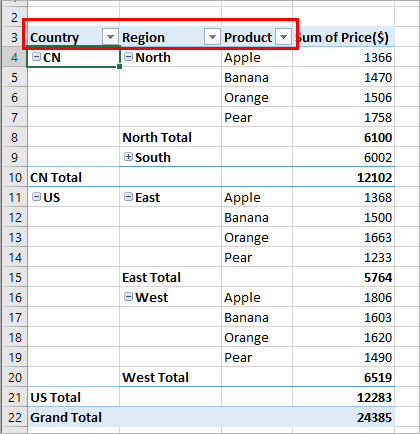
How to Concatenate Values of Pivot Table - Basic Excel Tutorial =CONCATENATE (C2, ", ", D2) Add a PivotTable with the combined address column Format the PivotTable to display the data in columns. Go to Pivot tools and click the design menu. On the layout group, choose report layout and select show in tabular form. The data will be displayed as shown below. Concatenate strings with a line break

Insert Blank Rows In a Pivot Table - Free Microsoft Excel Tutorials

Repeat item labels in a PivotTable - support.microsoft.com Right-click the row or column label you want to repeat, and click Field Settings. Click the Layout & Print tab, and check the Repeat item labels box. Make sure Show item labels in tabular form is selected. Notes: When you edit any of the repeated labels, the changes you make are applied to all other cells with the same label.

How to Sort Pivot Table Row Labels, Column Field Labels and Data Values with Excel VBA Macro ...

Grouping Pivot Row Labels - YouTube Grouping Pivot Row Labels - YouTube. About Press Copyright Contact us Creators Advertise Developers Terms Privacy Policy & Safety How YouTube works Test new features.

Pivot table row labels in separate columns • AuditExcel.co.za

Pivot Table Row Labels In the Same Line - Beat Excel! Then navigate to "Layout & Print" tab and click on "Show item in tabular form" option. Do this procedure also for "Dealer" field and your table will look like this: If you also want dealer names to repeat on each row, reopen "Dealer field settings and check "Repear item labels" option in "Layout & Print" tab.

Accelerate Your Analysis with Pivot Table | Simplified Excel

Πληροφοριακά Συστήματα Διοίκησης - Ανοικτά Ακαδημαϊκά ... 3.4.7 Pivot Table. ΑΣΚΗΣΗ. Επεξεργαστείτε τον παρακάτω πίνακα με τη χρήση Pivot Table. date of sales. Employee. Name. Item Sold. Quantity Sold. Euro Amount.102 σελίδες

Probably a better way: Visual display with pivot tables – Excel VBA

Spreadsheets: Problems with Pivot Table Labels - CFO To return to a normal layout of the pivot table, follow these steps: 1. Select any cell inside the pivot table. The PivotTable Tools tabs appear in the Ribbon. 2. Go to Design tab of the ribbon. 3. From the Design tab, open the Report Layout dropdown. 4.

Excel Pivot Table Combine Columns | Decoration Items Image

Pivot table row labels side by side - Excel Tutorials Now, let's create a pivot table ( Insert >> Tables >> Pivot Table) and check all the values in Pivot Table Fields. Fields should look like this. Right-click inside a pivot table and choose PivotTable Options…. Check data as shown on the image below. The table is going to change. The pivot table is almost ready.