44 align data labels in excel chart
Best Types of Charts in Excel for Data Analysis ... - Optimize Smart To add a chart to an Excel spreadsheet, follow the steps below: Step-1: Open MS Excel and navigate to the spreadsheet, which contains the data table you want to use for creating a chart. Step-2: Select data for the chart: Step-3: Click on the 'Insert' tab: Step-4: Click on the 'Recommended Charts' button: › toolsExcel Tools and Utilities Move and align chart titles, labels, legends with the arrow keys and alignment buttons. Absolute Reference Add-in Quickly create absolute references for table formulas (structured references) using the F4 key.
SAS Help Center Use PROC CONTENTS to view the contents of the data set before removing the labels and format. proc contents data=mylib.class; run; Within PROC DATASETS, remove all the labels and formats using the MODIFY statement and the ATTRIB option. Use the CONTENTS statement within PROC DATASETS to view the contents of the data set without the labels and ...
Align data labels in excel chart
How to Convert Excel Columns and Rows (Step by Step) Shift-click the last cell of the range. Your data set should highlight. From the Home tab, select Copy or type Ctrl + c. Pin. Copying the current Excel data. Select the new cell where you would like to copy your transposed data. Right-click in that cell and select the Transpose icon from the Paste Options. Pin. How to use Table Spreadsheet macro - StiltSoft Docs - Table Filter and ... Adding the Table Spreadsheet macro. 1. Insert the macro on a page: Start entering /Table Spreadsheet and select the macro. On the editor pane, click Insert -> View more, find the macro and insert it on the page Excel Slicer And Timeline - Tutorial With Examples How To Create Timeline In Excel. Click anywhere on the Pivot table, and the PivotTable Tools ribbon will be displayed. Go to PivotTable Tools -> Analyze -> Insert Timelines. Click on Insert Timeline. Insert Timeline dialog which will only show the date column of your table will appear. Select the date checkbox.
Align data labels in excel chart. How to smooth out a plot in excel to get a curve instead of scattered ... Click anywhere in the chart. On the Chart Design tab of the ribbon, click Add Chart Element > Trendline > More Trendline Options... Select Moving Average, then set the Period to (for example) 100. Play with the value of Period to see if you get something you like. Questions from Tableau Training: Can I Move Mark Labels? Option 1: Label Button Alignment. In the below example, a bar chart is labeled at the rightmost edge of each bar. Navigating to the Label button reveals that Tableau has defaulted the alignment to automatic. However, by clicking the drop-down menu, we have the option to choose our mark alignment. How to: Display and Format Data Labels - DevExpress When data changes, information in the data labels is updated automatically. If required, you can also display custom information in a label. Select the action you wish to perform. Add Data Labels to the Chart. Specify the Position of Data Labels. Apply Number Format to Data Labels. Create a Custom Label Entry. peltiertech.com › text-labels-on-horizontal-axis-in-eText Labels on a Horizontal Bar Chart in Excel - Peltier Tech Dec 21, 2010 · In Excel 2003 the chart has a Ratings labels at the top of the chart, because it has secondary horizontal axis. Excel 2007 has no Ratings labels or secondary horizontal axis, so we have to add the axis by hand. On the Excel 2007 Chart Tools > Layout tab, click Axes, then Secondary Horizontal Axis, then Show Left to Right Axis.
Vertical stacked bar charts in Excel - Microsoft Tech Community Hi. I've created this chart in Excel and want to make the entries in the legend appear in the same order top to bottom as they are in the chart (the legend reads A to D from the top but the bars read A to D from the bottom). I tried the following: Right-click on one of the names listed on your legend. Free Label Templates for Creating and Designing Labels Maestro Label Designer. Maestro Label Designer is online label design software created exclusively for OnlineLabels.com customers. It's a simplified design program preloaded with both blank and pre-designed templates for our label configurations. It includes a set of open-sourced fonts, clipart, and tools - everything you could need to create ... Gender Statistics | DataBank Create. Share: Development Data. DataBank is an analysis and visualisation tool that contains collections of time series data on a variety of topics. You can create your own queries; generate tables, charts, and maps; and easily save, embed, and share them. Enjoy using DataBank and let us know what you think! superuser.com › questions › 188064Excel chart with two X-axes (horizontal), possible? - Super User A 3D column chart may accommodate the data, but not in a way that makes it at all intelligible. This would most likely be best as an XY Scatter chart, with two series: one using regular X values, the other using normalized X values, and both using the same Y values. After adding the secondary horizontal axis, delete the secondary vertical axis.
Excel table styles and formatting: how to apply, change and remove On the Design tab, in the Table Styles group, click the More button. Underneath the table style templates, click Clear. Tip. To remove a table but keep data and formatting, go to the Design tab Tools group, and click Convert to Range. Or, right-click anywhere within the table, and select Table > Convert to Range. Excel: Group rows automatically or manually, collapse and ... - Ablebits To remove grouping for certain rows without deleting the whole outline, do the following: Select the rows you want to ungroup. Go to the Data tab > Outline group, and click the Ungroup button. Or press Shift + Alt + Left Arrow which is the Ungroup shortcut in Excel. In the Ungroup dialog box, select Rows and click OK. Sorting Data - SPSS Tutorials - LibGuides at Kent State University Click Data > Sort Cases. Double-click on the variable (s) you want to sort your data by to move them to the Sort by box. If you are sorting by two or more variables, then the order that the variables appear in the "Sort by" list matters. You can click and drag the variables to reorder them within the Sort by box. linkedin-skill-assessments-quizzes/microsoft-excel-quiz.md at ... - GitHub Q43. The charts below are based on the data in cells A3:G5. The chart on the right was created by copying the one on the left. Which ribbon button was clicked to change the layout of the chart on the right? Move Chart; Switch Row/Column; Quick Layout; Change Chart Type; Q44. Cell A20 displays an orange background when its value is 5.
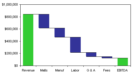
Excel 2016 charts: How to use the new Pareto, Histogram, and Waterfall ...
10 Core Formatting Techniques in Excel: Free Excel Tutorial 3) Resize Columns and Rows. a) Specify exact size. HOME >> Cells Group >> Format >> Row Width/Column Height or use the Right Click menu. b) Autofit. Double click on the line separating two column letters. or use HOME >> Cells Group >> Format >> Autofit. c) Drag to adjust. Click on the line separating two columns and drag left or right, as desired.
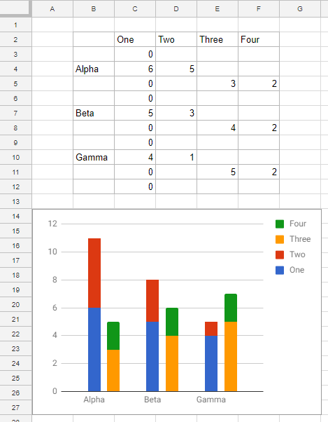
Clustered and Stacked Column and Bar Charts - Peltier Tech
Use defined names to automatically update a chart range - Office On the Insert tab, click a chart, and then click a chart type. Click the Design tab, click the Select Data in the Data group. Under Legend Entries (Series), click Edit. In the Series values box, type =Sheet1!Sales, and then click OK. Under Horizontal (Category) Axis Labels, click Edit. In the Axis label range box, type =Sheet1!Date, and then ...
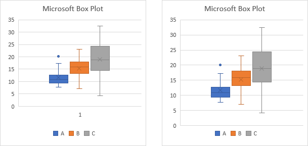
A Comparison of Peltier Tech and Excel Box Plots - Peltier Tech Blog
50 Excel Shortcuts That You Should Know in 2022 - Simplilearn Ctrl + Shift + Up Arrow. 25. To select all the cells below the selected cell. Ctrl + Shift + Down Arrow. In addition to the above-mentioned cell formatting shortcuts, let's look at a few more additional and advanced cell formatting Excel shortcuts, that might come handy. We will learn how to add a comment to a cell.

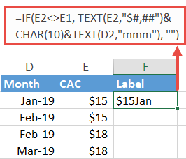
» Excel Charts: Creating Custom Data Labels
How to: Display and Format Data Labels - DevExpress Add Data Labels to the Chart; Specify the Position of Data Labels; Apply Number Format to Data Labels; Create a Custom Label Entry; Add Data Labels to the Chart. Basic settings that specify the contents, position and appearance of data labels in the chart are defined by the DataLabelOptions object, accessed by the ChartView.DataLabels property ...

How to Make Excel Charts More Intuitive by Adding Data Labels and ...
Chart Studies - Sierra Chart Chart Studies. A simple definition of a Study is that it is a graph of the results from a formula applied to the entire series of data elements in a chart. A study may also be called an indicator. In Sierra Chart they are called studies. See the Technical Studies Reference documentation page for information on the available studies. In Sierra Chart, you can also create your own custom study by ...

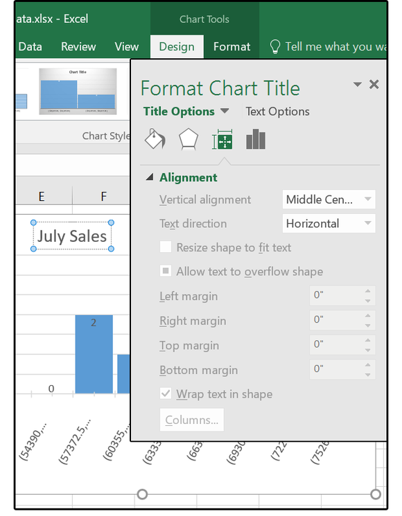
Microsoft Excel Tutorials: The Chart Title and Series Title
Control settings in the Format Cells dialog box - Office Text data is left-aligned, and numbers, dates, and times are right-aligned. Changing the alignment does not change the type of data. Left (Indent) Aligns contents at the left edge of the cell. If you specify a number in the Indent box, Microsoft Excel indents the contents of the cell from the left by the specified number of character spaces.
How to Create a Step Chart in Excel - Automate Excel
Angular 9|8|7 Material Table Column Width, Text Alignment Customization Install Angular Material. After creating the project, install the Material package in the project to use data-table component UI. Run the following command to install the Material package by answering a few questions: $ ng add @angular/material ? Choose a prebuilt theme name, or "custom" for a custom theme: Indigo/Pink ?

Excel chart not printing correctly - i have a simple excel file (office
How to Create Charts in Excel: Types & Step by Step Examples Below are the steps to create chart in MS Excel: Open Excel. Enter the data from the sample data table above. Your workbook should now look as follows. To get the desired chart you have to follow the following steps. Select the data you want to represent in graph. Click on INSERT tab from the ribbon. Click on the Column chart drop down button.
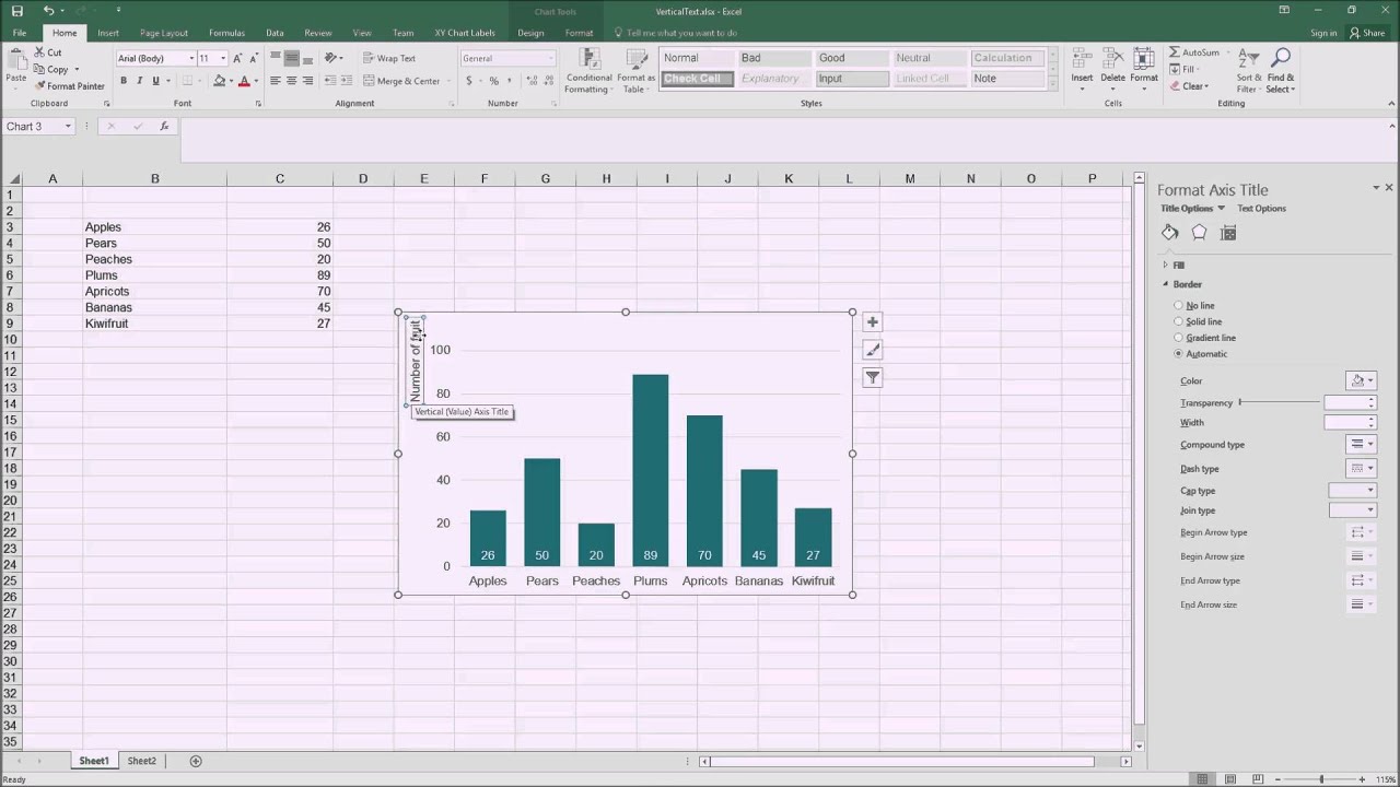
Adding horizontally-aligned y-axis titles to charts in Excel 2016 - YouTube
Questions from Tableau Training: Moving Reference Line Labels Formatting Labels in Tableau. For starters, right-click directly on top of your reference line and select Format. This will open a pane on the left where our Data and Analytics panes usually are. Here we can change how our reference line appears, similar to the options when we first create our reference line. More relevant here are the changes ...

Format Excel Data Before Running Charts | QI Macros
Blank Labels on Sheets for Inkjet/Laser | Online Labels® Nice labels as usual. Item: OL3282WX - 3.5" Circle Labels | Standard White Matte (Laser and Inkjet) By Kristi on May 2, 2022. These work great in our printer without any jams, and the art lines up with the template. What more could you ask for.

Enable or Disable Excel Data Labels at the click of a button - How To ...
› custom-data-labels-in-xImprove your X Y Scatter Chart with custom data labels May 06, 2021 · Thank you for your Excel 2010 workaround for custom data labels in XY scatter charts. It basically works for me until I insert a new row in the worksheet associated with the chart. Doing so breaks the absolute references to data labels after the inserted row and Excel won't let me change the data labels to relative references.
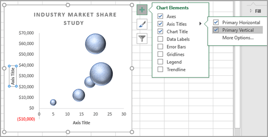
Present your data in a bubble chart - Excel
Chart Types - Data Visualization - Guides at University of Guelph Note, see histograms for continuous data.; Data. One (or more) text (categorical) variable; One numerical variable; Strength. Familiar to most audiences; High perceptual accuracy because they use alignment and length; Best practices. Use horizontal bars to enhance label readability; Consider sorting bars by length when alphabetical order is not ...

Excel Charts Archives - PakAccountants.com
How to fetch data from localserver database and display on HTML table ... PHP is used to connect with the localhost server and to fetch the data from the database table present in our localhost server by evaluating the MySQL queries. Wampserver helps to start Apache and MySQL and connect them with the PHP file. Consider, we have a database named gfg, a table named userdata. Now, here is the PHP code to fetch data ...
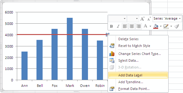
How To Add an Average Line to Column Chart in Excel 2010 - Excel How To
How to Change the Y Axis in Excel - Alphr In your chart, click the "Y axis" that you want to change. It will show a border to represent that it is highlighted/selected. Click on the "Format" tab, then choose "Format Selection ...

Display Data and Percentage in Pie Chart | SAP Blogs
ppcexpo.com › blog › how-to-analyze-likert-scale-dataHow to Analyze Likert Scale Data in Microsoft Excel and ... You can explore the sample data of the chart by clicking on the ‘Add Sample Chart + Data’. Let us see an example of how Curtis visualized his Likert scale data. Curtis runs a software company.
Add Percentages on the Secondary Axis - Peltier Tech Blog
andypope.info › chartsChart section - AJP Excel Information A worked example of a column chart with a break in the value axis. Display data with large variance between min and max values More ...
Post a Comment for "44 align data labels in excel chart"