41 excel pie chart with lines to labels

How to add Axis Labels (X & Y) in Excel & Google Sheets This tutorial will explain how to add Axis Labels on the X & Y Axis in Excel and Google Sheets. How to Add Axis Labels (X&Y) in Excel. Graphs and charts in Excel are a great way to visualize a dataset in a way that is easy to understand. The user should be able to understand every aspect about what the visualization is trying to show right away ... How To Make A Pie Chart In Excel: In Just 2 Minutes [2022] When you first create a pie chart, Excel will use the default colors and design.. But if you want to customize your chart to your own liking, you have plenty of options. The easiest way to get an entirely new look is with chart styles.. In the Design portion of the Ribbon, you’ll see a number of different styles displayed in a row. Mouse over them to see a preview:

› charts › timeline-templateHow to Create a Timeline Chart in Excel – Automate Excel Right-click on any of the columns representing Series “Hours Spent” and select “Add Data Labels.” Once there, right-click on any of the data labels and open the Format Data Labels task pane. Then, insert the labels into your chart: Navigate to the Label Options tab. Check the “Value From Cells” box.

Excel pie chart with lines to labels

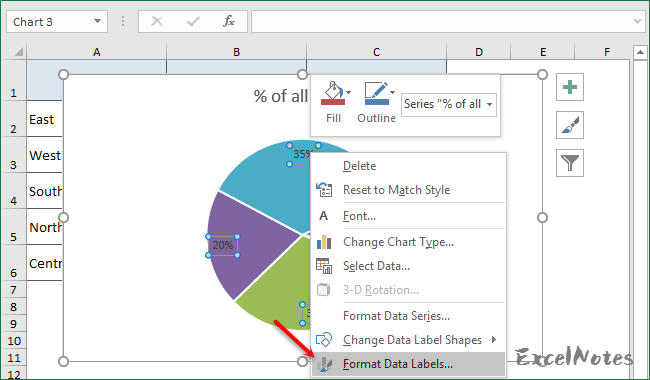
Advanced Excel - Leader Lines - Tutorialspoint Step 1 − Click on the data label. Step 2 − Drag it after you see the four-headed arrow. Step 3 − Move the data label. The Leader Line automatically adjusts and follows it. Format Leader Lines Step 1 − Right-click on the Leader Line you want to format. Step 2 − Click on Format Leader Lines. The Format Leader Lines task pane appears. Excel charts: add title, customize chart axis, legend and data labels ... To change what is displayed on the data labels in your chart, click the Chart Elements button > Data Labels > More options… This will bring up the Format Data Labels pane on the right of your worksheet. Switch to the Label Options tab, and select the option (s) you want under Label Contains: › documents › excelHow to show percentage in pie chart in Excel? - ExtendOffice 1. Select the data you will create a pie chart based on, click Insert > Insert Pie or Doughnut Chart > Pie. See screenshot: 2. Then a pie chart is created. Right click the pie chart and select Add Data Labels from the context menu. 3. Now the corresponding values are displayed in the pie slices. Right click the pie chart again and select Format ...

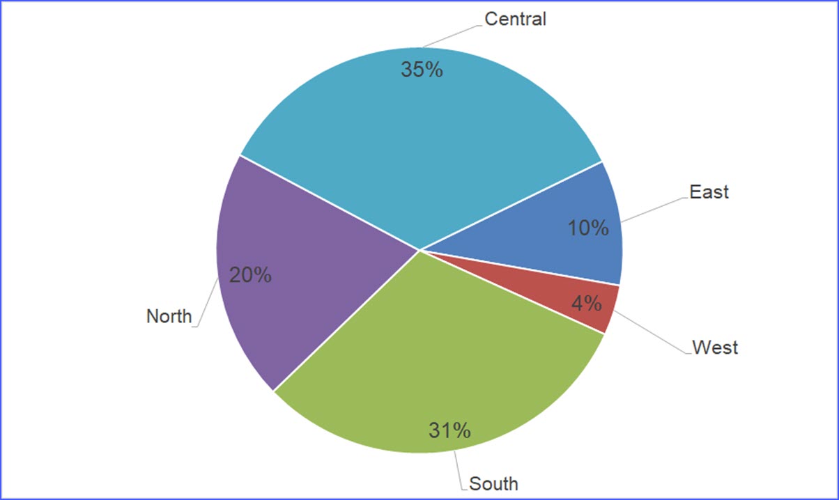
Excel pie chart with lines to labels. How to display leader lines in pie chart in Excel? 1. Click at the chart, and right click to select Format Data Labels from context menu. 2. In the popping Format Data Labels dialog/pane, check Show Leader Lines in the Label Options section. See screenshot: 3. Close the dialog, now you can see some leader lines appear. If you want to show all leader lines, just drag the labels out of the pie ... Display data point labels outside a pie chart in a paginated report ... The PieLineColor property defines callout lines for each data point label. To prevent overlapping labels displayed outside a pie chart. Create a pie chart with external labels. On the design surface, right-click outside the pie chart but inside the chart borders and select Chart Area Properties.The Chart AreaProperties dialog box appears. On ... Microsoft Excel Tutorials: Add Data Labels to a Pie Chart The chart is selected when you can see all those blue circles surrounding it. Now right click the chart. You should get the following menu: From the menu, select Add Data Labels. New data labels will then appear on your chart: The values are in percentages in Excel 2007, however. To change this, right click your chart again. How to Create Pie Charts in Excel (In Easy Steps) Click the + button on the right side of the chart and click the check box next to Data Labels. 10. Click the paintbrush icon on the right side of the chart and change the color scheme of the pie chart. Result: 11. Right click the pie chart and click Format Data Labels. 12. Check Category Name, uncheck Value, check Percentage and click Center.

Leader lines for Pie chart are appearing only when the data labels are ... I have a pie chart with data labels connected to leader lines. Though I have set the position of labels to 'Outside End', the leader lines are not appearing by default. It shows up only when I manually move the data labels. I dont have to move them far apart. Just a slight change in the position of labels helps. Pie Charts how do you show Label and Value? - MrExcel Message Board Using a macro to add the values after the graph is drawn does not stay live - the graph may get re-drawn to the correct proportions but the label won't change unless the macro is re-run. It does seem from some of the above replies that some versions of Excel allow you to select label and value - will try to find out later (can test up to 2002 ... How to Create a Pie Chart in Excel | Smartsheet To create a pie chart in Excel 2016, add your data set to a worksheet and highlight it. Then click the Insert tab, and click the dropdown menu next to the image of a pie chart. Select the chart type you want to use and the chosen chart will appear on the worksheet with the data you selected. Creating Pie Chart and Adding/Formatting Data Labels (Excel) Creating Pie Chart and Adding/Formatting Data Labels (Excel)

Rotate charts in Excel - spin bar, column, pie and line charts ... 09.07.2014 · I think 190 degrees will work fine for my pie chart. After being rotated my pie chart in Excel looks neat and well-arranged. Thus, you can see that it's quite easy to rotate an Excel chart to any angle till it looks the way you need. It's helpful for fine-tuning the layout of the labels or making the most important slices stand out. Rotate 3-D ... How to make a pie chart in Excel - ablebits.com Adding data labels to Excel pie charts. In this pie chart example, we are going to add labels to all data points. To do this, click the Chart Elements button in the upper-right corner of your pie graph, and select the Data Labels option. Additionally, you may want to change the Excel pie chart labels location by clicking the arrow next to Data ... Adding 2nd Data Label Series to Bar of Pie Chart If you use 2 sets of the same data in the chart you can create 2 pie/bar charts, with one appearing on the secondary axis. Make sure the settings for bar/pie formatting are the same. Add data labels to each series. Format one to show names the other values. Within the pie you may want to delete the name data labels. Attached Files How to Create Bar of Pie Chart in Excel? Step-by-Step Pie charts in Excel provide a great way to visualize categorical data as part of a whole. By one look at a pie chart, one can tell how much a category contributes to the entire group. A bar of pie chart lets us go one step further and helps us visualize pie charts that are a little more complex.

Show mini trend charts for large reports • Online-Excel-Training.AuditExcel.co.za

Change the format of data labels in a chart To get there, after adding your data labels, select the data label to format, and then click Chart Elements > Data Labels > More Options. To go to the appropriate area, click one of the four icons ( Fill & Line, Effects, Size & Properties ( Layout & Properties in Outlook or Word), or Label Options) shown here.

Tableau Bar Chart Labels Overlapping - Free Table Bar Chart

Create a pie chart from distinct values in one column by grouping … On the PivotTable Field List drag Country to Row Labels and Count to Values if Excel doesn't automatically. Now select the pivot table data and create your pie chart as usual. P.S. I use the pivot table for I update the data on a regular basis, then I just replace the "Country" data and refresh the pivot table.

How to Make Pie Chart with Labels both Inside and Outside - ExcelNotes

Excel 2010 pie chart data labels in case of "Best Fit" Based on my tested in Excel 2010, the data labels in the "Inside" or "Outside" is based on the data source. If the gap between the data is big, the data labels and leader lines is "outside" the chart. And if the gap between the data is small, the data labels and leader lines is "inside" the chart. Regards, George Zhao. TechNet Community Support.

How-to Make a WSJ Excel Pie Chart with Labels Both Inside and Outside - Excel Dashboard Templates

How to show percentage in pie chart in Excel? - ExtendOffice Show percentage in pie chart in Excel. Please do as follows to create a pie chart and show percentage in the pie slices. 1. Select the data you will create a pie chart based on, click Insert > Insert Pie or Doughnut Chart > Pie. See screenshot: 2. Then a pie chart is created. Right click the pie chart and select Add Data Labels from the context ...

How to display leader lines in pie chart in Excel?

Dynamically Label Excel Chart Series Lines - My Online Training Hub Label Excel Chart Series Lines One option is to add the series name labels to the very last point in each line and then set the label position to 'right': But this approach is high maintenance to set up and maintain, because when you add new data you have to remove the labels and insert them again on the new last data points.

How To Make A Cashier Count Chart In Excel - 31 How To Label Pie Charts In Excel - Labels ...

› tutorials › create-family-treeHow to Create a Family Tree Chart in Excel, Word, Numbers ... Step 1: Create a New Spreadsheet. Launch a new Excel document by clicking the start button, and then click on Microsoft Office to select Microsoft Excel Templates.Once all that is done, click File from the menu and click New to select a template to create a family tree.

How to Make Pie Chart with Labels both Inside and Outside - ExcelNotes

How-to Add Label Leader Lines to an Excel Pie Chart - YouTube Step-by-Step Tutorial: how-to create label leader lines that connect pie labels that are outsi...

components - What can I use to implement a doughnut chart in iOS? - Stack Overflow

Tableau Pie Chart Label Lines - TheRescipes.info Dynamic Exterior Pie Chart Labels with Arrows/lines - Tableau trend kb.tableau.com. Answer As a workaround, use Annotations: Select an individual pie chart slice (or all slices). Right-click the pie, and click on Annotate > Mark.Edit the dialog box that pops up as needed to show the desired fields, then click OK.

Share :